Table of Contents
Introduction
Understanding Time Series Data
Project Overview
Data Preparation
Loading and Inspecting the Data
Visualizing the Data
5. Feature Engineering
Extracting Time-Based Features
Implementing Feature Engineering
6. Model Training with XGBoost
Splitting the Data
Training the XGBoost Model
7. Model Evaluation and Forecasting
Evaluating the Model
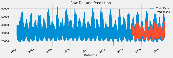
Visualizing Predictions
8. Deploying with Streamlit
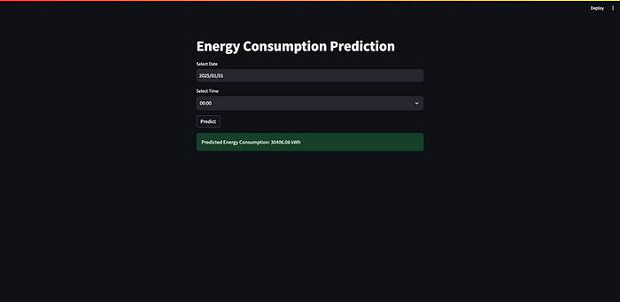
Creating the Streamlit App
Running the Application
9. Conclusion and Next Steps
1. Introduction
In the world of data science, time series forecasting is a crucial technique used to predict future values based on historical data. It is widely applied in various domains such as finance, weather prediction, and energy consumption. In this blog, we’ll explore how to predict energy consumption using time series forecasting with the XGBoost machine learning model. We’ll go through the steps of preparing the data, engineering features, training the model, and finally deploying the model using a Streamlit interface.
2. Understanding Time Series Data
Time series data consists of sequential observations recorded over time. Unlike regular datasets, time series data carries a temporal ordering which is crucial for analysis. The data often displays trends (long-term increase or decrease), seasonality (repeating patterns), and cycles (fluctuations at irregular intervals). Understanding these patterns is essential for accurate forecasting.
3. Project Overview
In this project, we aim to predict hourly energy consumption for a specific region using a historical dataset that spans over a decade. The project involves the following steps:
Data Preparation: Load and clean the data, ensuring it’s in a suitable format for analysis.
Feature Engineering: Extract meaningful features from the data to help the model learn better.
Model Training: Train an XGBoost model on the data to forecast future energy consumption.
Model Evaluation: Assess the model’s performance using appropriate metrics and visualizations.
Deployment: Use Streamlit to create a user-friendly web application for making predictions.
4. Data Preparation
Loading and Inspecting the Data
We start by loading the dataset using Pandas. The dataset contains hourly energy consumption records with a Datetime column representing the timestamp.
import pandas as pd
# Load the dataset
df = pd.read_csv('energy_dataset/PJME_hourly.csv')
df.head()
The first few rows of the dataset give us a glimpse into its structure:
Datetime    PJME_MW
0   2002-01-01 01:00:00  5087.546
1   2002-01-01 02:00:00  5050.118
2   2002-01-01 03:00:00  4993.485
3   2002-01-01 04:00:00  4919.263
4   2002-01-01 05:00:00  4865.211
Next, we set the Datetime column as the index and convert it to a datetime type for easier manipulation.
# Convert Datetime to datetime type and set as index
df['Datetime'] = pd.to_datetime(df['Datetime'])
df = df.set_index('Datetime')
Visualizing the Data
Visualizing the data helps us understand its trends and seasonality. We can plot the entire time series to observe the patterns over time.
import matplotlib.pyplot as plt
# Plot the time series data
plt.figure(figsize=(10, 6))
df['PJME_MW'].plot(title='Energy Consumption Over Time')
plt.show()
The plot shows how energy consumption fluctuates over time, with noticeable seasonal patterns corresponding to different times of the year.
5. Feature Engineering
Extracting Time-Based Features
To improve our model’s performance, we create new features that capture the temporal aspects of the data. For example, the hour of the day, day of the week, and month can all provide valuable information.
def create_features(df):
    """
    Create time series features based on time series index.
    """
    df = df.copy()
    df['hour'] = df.index.hour
    df['dayofweek'] = df.index.dayofweek
    df['quarter'] = df.index.quarter
    df['month'] = df.index.month
    df['year'] = df.index.year
    df['dayofyear'] = df.index.dayofyear
    df['dayofmonth'] = df.index.day
    df['weekofyear'] = df.index.isocalendar().week
    return df
These features help the model recognize patterns, such as higher energy consumption during certain hours or seasons.
Implementing Feature Engineering
To streamline the feature engineering process, we encapsulate it in a function. This function adds all the relevant features to the DataFrame.
# Apply the feature creation function
df = create_features(df)
Now our dataset includes the engineered features, which will be used in the model training process.
6. Model Training with XGBoost
Splitting the Data
Before training the model, we split the dataset into training and test sets. This allows us to train the model on historical data and evaluate its performance on unseen data.
# Split the data into training and test sets
train = df.loc[df.index < '2015-01-01']
test = df.loc[df.index >= '2015-01-01']
Training the XGBoost Model
XGBoost is a powerful algorithm known for its speed and performance. We use it to train a regression model to predict energy consumption.
import xgboost as xgb
from sklearn.metrics import mean_squared_error
# Define features and target
features = ['hour', 'day_of_week', 'month', 'year']
X_train = train[features]
y_train = train['PJME_MW']
X_test = test[features]
y_test = test['PJME_MW']
# Initialize and train the model
model = xgb.XGBRegressor(n_estimators=1000, early_stopping_rounds=50, learning_rate=0.01)
model.fit(X_train, y_train, eval_set=[(X_test, y_test)], verbose=100)
The model is trained using the features we created, with the number of estimators and learning rate adjusted to optimize performance.
7. Model Evaluation and Forecasting
Evaluating the Model
Once the model is trained, we evaluate its performance using the Root Mean Squared Error (RMSE), which penalizes large errors.
# Predict on the test set
y_pred = model.predict(X_test)
# Calculate RMSE
rmse = mean_squared_error(y_test, y_pred, squared=False)
print(f'RMSE: {rmse}')
The RMSE provides a quantitative measure of how well the model is performing on the test set.
Visualizing Predictions
Visualizing the predictions alongside the actual data helps us see how closely the model’s predictions align with reality.
# Plot predictions vs actual
plt.figure(figsize=(10, 6))
plt.plot(test.index, y_test, label='Actual')
plt.plot(test.index, y_pred, label='Predicted', color='red')
plt.legend()
plt.title('Energy Consumption: Actual vs Predicted')
plt.show()

This plot allows us to visually inspect the model’s performance, highlighting areas where the predictions are accurate and where improvements might be needed.
8. Deploying with Streamlit
Creating the Streamlit App
To make our model accessible to users, we deploy it using Streamlit, which provides an easy-to-use interface for building web applications.
import streamlit as st
import pandas as pd
import numpy as np
from datetime import datetime
import pickle
from functions import predict_energy
# Load the pre-trained model
loaded_model = pickle.load(open('time_series_model.sav', 'rb'))# Streamlit UI
st.title('Energy Consumption Prediction')# Input: Date and Time using Streamlit's date_input and time_input
selected_date = st.date_input('Select Date')
selected_time = st.time_input('Select Time')# Combine selected date and time into a datetime object
if selected_date and selected_time:
    date_time_obj = datetime.combine(selected_date, selected_time)if st.button('Predict'):
    try:
        prediction = predict_energy(date_time_obj,loaded_model)
        st.success(f'Predicted Energy Consumption: {prediction:.2f} kWh')
    except Exception as e:
        st.error(f"Error: {e}")
This Streamlit app allows users to input a date and time, and get the predicted energy consumption for that specific moment.
Running the Application
To run the Streamlit app, simply execute the following command:
streamlit run app.py
This will start a local web server and open the app in your browser, providing a simple yet powerful interface for interacting with the model.

9. Conclusion and Next Steps
In this project, we successfully predicted energy consumption using time series forecasting and XGBoost. We went through the entire process of data preparation, feature engineering, model training, and deployment. While the model performs well, there are always opportunities for improvement, such as adding more features or fine-tuning the model’s hyperparameters.
As a next step, consider exploring additional data sources like weather information or special events, which could further enhance the model’s accuracy.

