


1. Introduction
Medical image classification is one of the most important problems in the image recognition area, and its aim is to classify medical images into different categories to help doctors in disease diagnosis or further research. Overall, medical image classification can be divided into two steps. The first step is extracting effective features from the image. The second step is using the features to build models that classify the image dataset. In the past, doctors usually used their professional experience to extract features to classify the medical images into different classes, which is usually a difficult, and time-consuming task.
Considering the advancement in machine learning, Deep learning-based methods, which are the most breathtaking branch in AI ,provide an effective way to construct an end-to-end model that can compute final classification labels with the raw pixels of medical images.
In this article I will write about how Image classification model using CNN can be used to used to classify the healthy MRI image from a tumorous MRI image .
2. Steps Involved
Any Supervised learning starts with data collection.In this case we need to collect the images of healthy MRI images and MRI images with tumors. I have downloaded the required dataset from Kaggle: kaggle.com/datasets/navoneel/brain-mri-imag..
Data Cleaning and Preprocessing: We will perform Data scaling and Data augmentation in this step .Data augmentation is performed because we might have not have enough diverse of images so rotate , flip and adjust contrast to create more training sample.
Model Building: Convolutional Neural network is a standard way to do image classification. Here I have build a model using CNN.
2.1 Importing Libraries and dependencies
The required Libraries/dependencies are installed and imported in this step.
import numpy as np
import pandas as pd
import matplotlib.pyplot as plt

import tensorflow as tf
from tensorflow import keras
from tensorflow.keras import layers
from tensorflow.keras.models import Sequential
from tensorflow.keras.layers import Conv2D, MaxPooling2D, Dense, Flatten
from tensorflow.keras.metrics import BinaryAccuracy, Precision, Recall
import warnings
warnings.filterwarnings("ignore")
tf.keras.backend.clear_session()
2.2 Data Loading
We load the data by making use of the tool image_dataset_from directory. It helps us fetch the data from the relevant directory, automatically does labeling, shuffles the data, batches the data (in this case as 32) and resizes images into 256 by 256.
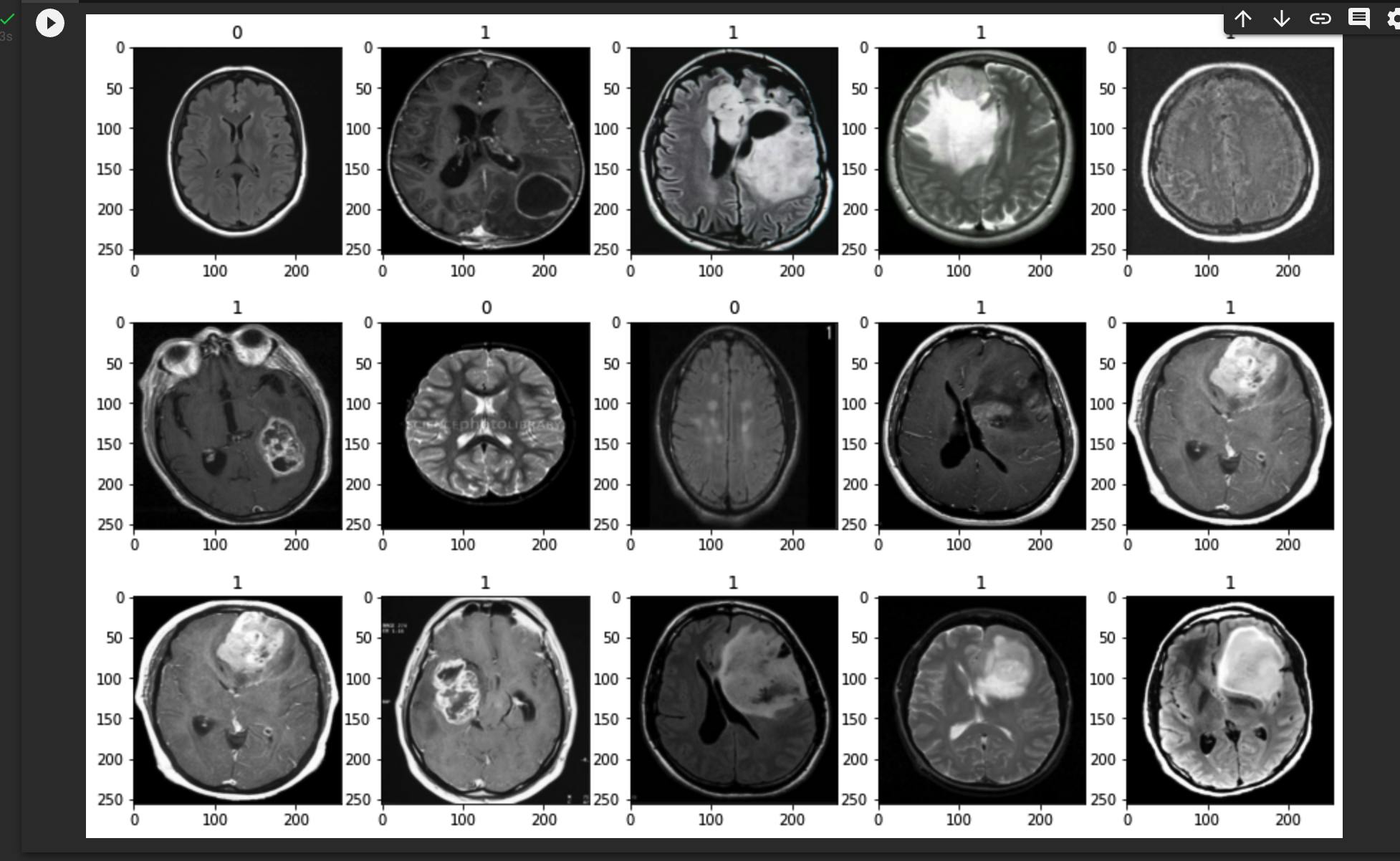
data = keras.utils.image_dataset_from_directory("/content/sample_data/MRI_Image_samples")

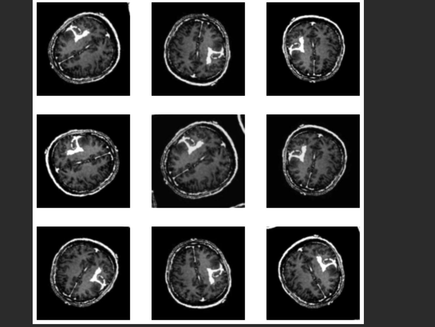
Plotting the loading Images
If a brain has tumor it is labeled as 1, if no it is labeled as 0.
batch = data.as_numpy_iterator().next()

fig, ax = plt.subplots(3, 5, figsize=(15,10))
ax = ax.flatten()
for idx, img in enumerate(batch[0][:15]):
    ax[idx].imshow(img.astype(int))
    ax[idx].title.set_text(batch[1][idx])
2.3 Data Preprocessing
Data preprocessing in Machine Learning is a crucial step that helps enhance the quality of data to promote the extraction of meaningful insights from the data. Data preprocessing in Machine Learning refers to the technique of preparing (cleaning and organizing) the raw data to make it suitable for a building and training Machine Learning models.
2.3.1 Data Scaling
Since our data consists of images and images consist of pixels, we divide all the pixel values by 255—each pixel can have a value in [0, 255]— so that all the pixel values are on the same scale i.e. [0, 1].
data = data.map(lambda x,y: (x/255, y))
batch = data.as_numpy_iterator().next()
print("Minimum value of the scaled data:", batch[0].min())
print("Maximum value of the scaled data:", batch[0].max())

2.3.2 Train-Validation-Test Split
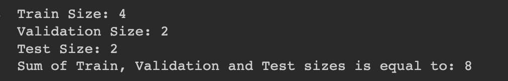
print("There are", len(data), "batches in our data")
Now, we have to divide the whole data into 3 separate sets: Train set for training the model, Validation set for adjusting the hyperparameters of our model and Test set for evaluating our model on the set that our model has not seen before. As it can be seen, we have 8 batches in our data. I preferred allocating 4 batches for Train set, 2 batches for Validation set and 2 batches for Test set.
train_size = int(len(data)*0.6)
val_size = int(len(data)*0.2)+1
test_size = int(len(data)*0.2)+1

print("Train Size:", train_size)
print("Validation Size:", val_size)
print("Test Size:", test_size)

print("Sum of Train, Validation and Test sizes is equal to:", train_size + val_size + test_size)
train = data.take(train_size)
val = data.skip(train_size).take(val_size)
test = data.skip(train_size + val_size).take(test_size)
2.3.3 Data Augmentation
Because our Train set has relatively small number of images, we can apply data augmentation which is reproducing the images by applying some changes such as random rotating, random flipping, random zoom and random contrast. This may possibly increase the accuracy score of the model. Since we will be applying the data augmentation in the beginning of the neural network architecture, we should pass the input shape.
batch = data.as_numpy_iterator().next()

data_augmentation = Sequential([
    layers.RandomFlip("horizontal_and_vertical", input_shape=(256,256,3)),
    layers.RandomZoom(0.1),
    layers.RandomContrast(0.1),
    layers.RandomRotation(0.2)
])

image = batch[0]


plt.figure(figsize=(10, 10))
for i in range(9):
    augmented_image = data_augmentation(image)
    ax = plt.subplot(3, 3, i + 1)
    plt.imshow(augmented_image[0])
    plt.axis("off")
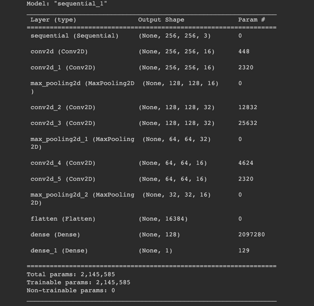
2.4 Model building
Now we are ready to build our model. The model type that we will be using is Sequential. Sequential is the easiest way to build a model in Keras. It allows you to build a model layer by layer.
model = Sequential([
    data_augmentation,
    Conv2D(16, (3,3), 1, activation="relu", padding="same"),
    Conv2D(16, (3,3), 1, activation="relu", padding="same"),
    MaxPooling2D(),
    Conv2D(32, (5,5), 1, activation="relu", padding="same"),
    Conv2D(32, (5,5), 1, activation="relu", padding="same"),
    MaxPooling2D(),
    Conv2D(16, (3,3), 1, activation="relu", padding="same"),
    Conv2D(16, (3,3), 1, activation="relu", padding="same"),
    MaxPooling2D(),

    Flatten(),
    Dense(128, activation="relu"),
    Dense(1, activation="sigmoid")
])
Next, we need to compile our model. Compiling the model takes three parameters: optimizer, loss and metrics.
The optimizer controls the learning rate. We will be using ‘adam’ as our optmizer. Adam is generally a good optimizer to use for many cases. The adam optimizer adjusts the learning rate throughout training.
The learning rate determines how fast the optimal weights for the model are calculated. A smaller learning rate may lead to more accurate weights (up to a certain point), but the time it takes to compute the weights will be longer.
We will use ‘crossentropy’ for our loss function. This is the most common choice for classification. A lower score indicates that the model is performing better.
To make things even easier to interpret, we will use the ‘accuracy’ metric to see the accuracy score on the validation set when we train the model.
model.compile(optimizer="adam", loss=keras.losses.BinaryCrossentropy(), metrics=["accuracy"])
model.summary()
history = model.fit(train, epochs=15, validation_data=val)
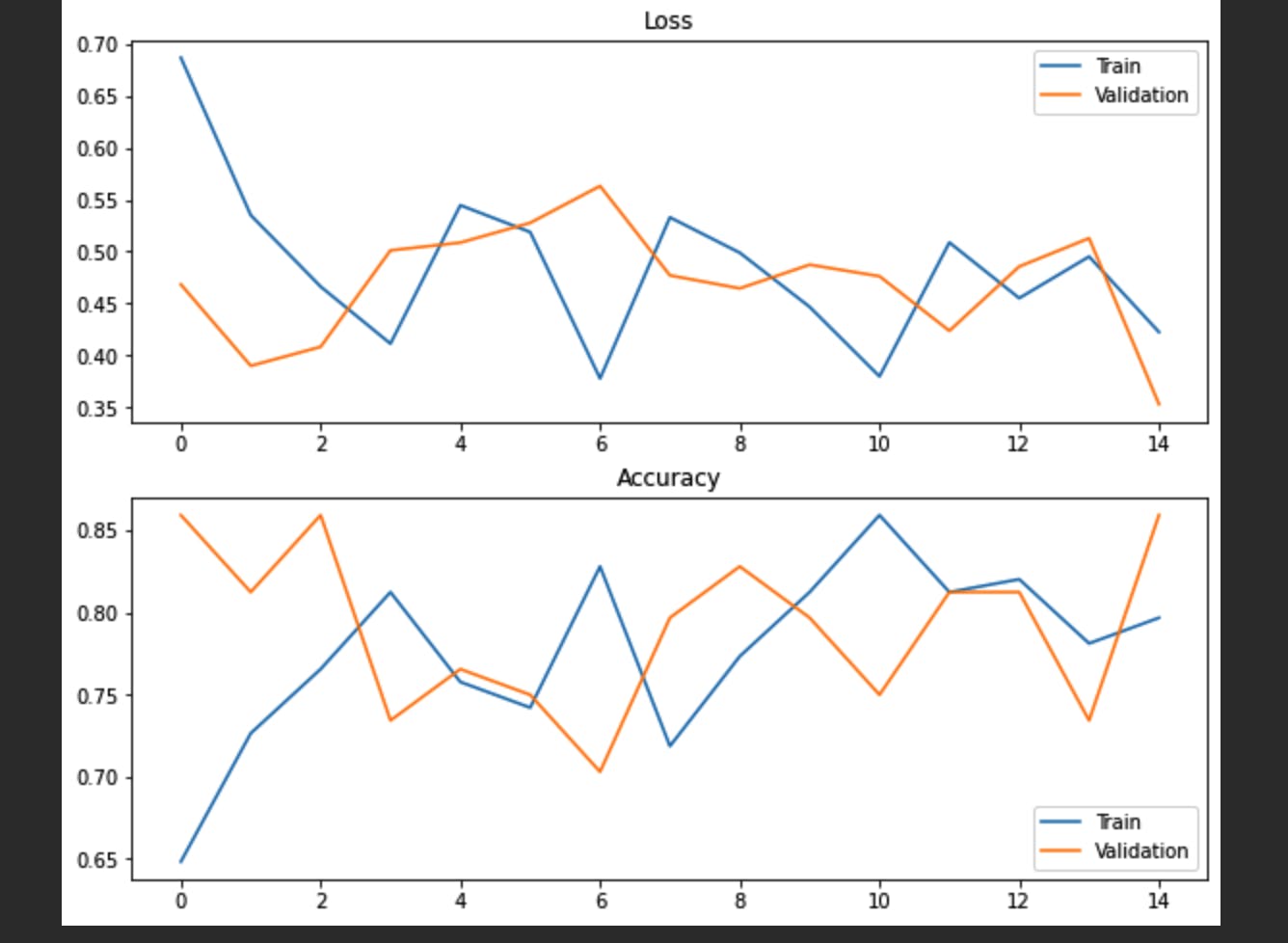
After 15 epochs, we have gotten to 79.69% accuracy on our validation set.That’s a very good start! Congrats, you have now built a CNN!.The accuracy can be further increased by parameter tuning.
2.4 Performance analysis
Here we evaluate the accuracy and loss of training and validation dataset over the No of epochs.
fig, ax = plt.subplots(2, 1, figsize=(10,8))

ax[0].plot(history.history["loss"], label="Train")
ax[0].plot(history.history["val_loss"], label="Validation")
ax[0].title.set_text("Loss")
ax[0].legend()

ax[1].plot(history.history["accuracy"], label="Train")
ax[1].plot(history.history["val_accuracy"], label="Validation")
ax[1].title.set_text("Accuracy")
ax[1].legend()

plt.show()
bin_acc = BinaryAccuracy()
recall = Recall()
precision = Precision()

for batch in test.as_numpy_iterator():
    X, y = batch
    yhat = model.predict(X)
    bin_acc.update_state(y, yhat)
    recall.update_state(y, yhat)
    precision.update_state(y, yhat)

print("Accuracy:", bin_acc.result().numpy(), "\nRecall:", recall.result().numpy(), "\nPrecision:", precision.result().numpy())

2.4 Testing
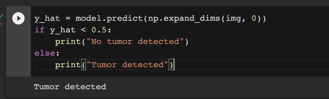
We have already evaluated our model using various metrics and visualizations but it is always a good practice to test the model by hand to make sure everything is working well. In the code below, I randomly chose an image and plotted it with its true label on title so let's see if our model is going to classify this example correctly.
batch = test.as_numpy_iterator().next()

img, label = batch[0][10], batch[1][10]
plt.imshow(img)
if label==1:
    plt.title("Brain with Tumor")
else:
    plt.title("Brain with No Tumor")
plt.show()
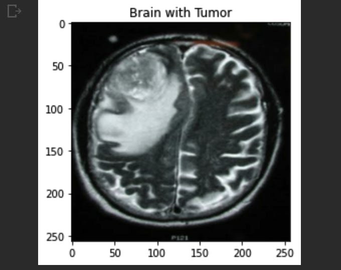
y_hat = model.predict(np.expand_dims(img, 0))
if y_hat < 0.5:
    print("No tumor detected")
else:
    print("Tumor detected")